NOTE: The examples in this essay currently only work in Chrome, and even then not in iOS. I'm working on it!

Introduction

This web essay will explore the addition of annotations and visualizations to custom-developed programming environments for live coding performance; in this essay I will use the term 'live coding' to refer to the digital arts practice, as opposed to live programming more generally. I provide a catalogue of techniques I've developed to help reveal algorithmic activity to both audience members and programmer/performers. These techniques are implemented in standard JavaScript, which is also the end-user language; however, many are generalizable and some have drawn inspiration from features found in programming environments for other languages. The code examples below are live; feel free to make minor edits and view / listen to the resulting changes. In addition to pressing the 'Play' button, which selects all code in a given example and runs it, you can also highlight code you'd like to execute and hit Ctrl+Enter.

Before diving in, I'd like to provide an example of what many of these annotations look like when combined, as shown in Listing 1. Although they might be somewhat overwhelming when simultaneously viewed, in my experience they can provide valuable scaffolding to the development of a program as it is written over time.

Catalog of techniques

This research augments programming interfaces to include visualizations, self-modifying source code, automated annotations via inserted code comments, and a variety of other techniques. By injecting annotations and visualizations into the source code itself, we improve association between code and the annotations / visualizations depicting its effects. This placement of visualizations is characterized as in situ by Hofswell et. al, [2], who demonstrated the effectiveness of such visualizations in improving both speed and accuracy when completing tasks related to data visualization and code comprehension.

Repeating static values

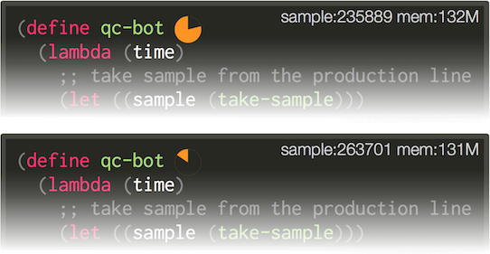
The simplest annotation added to our environment is a rotating border around static elements that are accessed repeatedly. The rotation provides a visual indication of when the values are used. Survey results indicated that rotation was preferable to other techniques (such as flashing) due to its less distracting nature [1].

Listing 2 shows a repeated scale index (0) being triggered every quarter note. We'll see how this simple annotation can be useful in combination with others in the next section.

It is worth noting that 'distracting' flashes can also be used to great effect; in the live-coding environment SchemeBricks by Dave Griffith blocks flash whenever they receive a control signal, providing an indication of activity with greater spectacle.

SLUB - Live coding from jomasan on Vimeo.

Cycling through musical patterns

Musical patterns (aka sets) are common ways of expressing lists that can be transformed and manipulated algorithmically. However, even if a pattern is read from start to finish without modification, it can still be useful to know which elements of the pattern are being triggered when, so that programmers and audience members can associate the the values being triggered with the corresponding sonic results.

In Listing 3, a synthesizer plays a simple pattern that loops through the seven notes of a standard scale from Western harmony. In addition to this melodic pattern, a rhythmic pattern alternates between quarter notes and eighth notes in duration.

The potential of this method is more apparent when the pattern is not playing sequentially. In Listing 4, scale indices are randomly chosen. Also note that the rotating border annotation now provides a indication of how many times a randomly chosen value has been repeated in a row (modulo 4).

Pattern transformations

20th-century serialist techniques transform musical pattern using many techniques, including reversal, rotation, inversion, and scaling. I was inspired by Thor Magnussons's ixi lang environment [3] to depict these transformations within the code itself, clearly revealing how patterns are transformed over time. The video below shows the effect of this technique in an ixi lang recreation of Steve Reich's composition Piano Phase.

ixi lang take on Steve Reich's Piano Phase from ixi audio on Vimeo.

In Listing 5, a percussion pattern is played against a steady kick drum rhythm. Each of the symbols in the percussion pattern denotes a different sound that is played; this pattern is then rotated one position after every measure, creating varying rhythms against the constant kick drum.

The code in Listing 5 is more complex than the previous examples in this essay, providing an opportunity to see how two different instruments rhythmically relate to each other and also view transformations in musical pattern. It is perhaps worth comparing the example given above to the exact same code without annotations, shown in Listing 6, in order to gauge how annotations affect perception of / engagement with code.

Revealing 'hidden' data and function output

As we saw from prior examples, we can highlight selected members of patterns as they are selected / triggered. However, this assumes that the pattern has been fully notated, with all its members included in the source code document. But it is natural to assume that in algorithmic music the source material for musical patterns will likely be defined algorithmically, as opposed to manually entered by a programmer/perfomer.

In such instances pattern generators are present in the source code as opposed to the data that they generate; the generated patterns are hidden. Our solution to this problem is to present these patterns in code comments adjacent to the code representing the pattern generators responsible for creating them. In Listing 7, we'll use a 'Euclidean' rhythm, a terse description of a rhythmic pattern drawn from a well-known musicology paper by Godfried Toussaint [3], where a given number of pulses are fit into a given number of slots using Bjorklund's algorithm. The results of running the Euclidean rhythm will determine the output of a kick drum. Whenever a zero is present in the pattern a rest will be triggered; a one (pulse) will trigger the kick drum.

These generated patterns can also be transformed over time, with the results depicted in the associated code comments. Note that when playback stops the code comments are automatically cleared. Listing 8 shows comments used to display both the initial data generated by the Euclidean rhythm and its subsequent transformations.

In contrast to defining patterns that are known ahead of time, it is also useful to generate values on-the-fly throughout performance; in our environments this can be done by passing functions that generate values to sequence constructors. The same technique we described earlier in this section for annotating generated patterns (shown in Listings 7–8) can also be used to show the output of such functions. Listing 9 shows the output of a function which outputs integers between 0-10; these values are then used to trigger notes in a scale.

We note that while Rndi (and Rndf) are included as convenience methods, there is nothing special about them in terms of annotations. The technique works for any function, enabling performers and students to experiment with writing their own generative functions while receiving visual feedback. Below we use an anonymous function that randomly returns a value of zero or one.

Visualizing continuous data

The previous examples have all featured data that is discrete; for example, notes are triggered at particular moments in time, as are pattern transformations and many other types of events. However, the musical world is divided into discrete and continuous data. An individual note might begin in a single moment but the expressive characteristics of that note, such as vibrato, are determined continuously over the note's duration.

During the development of gibberwocky, a live coding environment that targets external musical applications, my collaborator Graham Wakefield and I added affordances for defining continuous signals and sequencing changes to their parameters over time. In some live coding performances, I noticed that I often spent time at the beginning programming discrete events and patterns, and then segued to creating continuous manipulations of these events. Put another way, many performances consisted of initially creating patterns, and then subsequently adding expressive nuance to them. However, at the time there were no affordances in our environment for displaying continuous signals, which led to a suddent lack of visual feedback during performances when continuous controls were being programmed. In order to correct this we added a simple visualization showing the output of generated signals. In Listing 11, the cutoff frequency of a resonant filter is controller by a sine oscillator.

Although we initially used sparklines for these visualizations, we subsequently found that including the output range of the signals greatly improved their usefulness. One interesting point to note is that the output ranges are dynamic, based off an analysis of the generated signal. This means that if the signal range changes by a significant factor, the visualization will update itself to reflect the current average output range; this behavior can be seen in the first example found in this essay.

However, for certain types of signals portraying the current window and its adjusted range proves problematic. Consider the ambient piece presented below, created using gibberwocky by performer Lukas Nowok. The piece primarily consists of long gestures, many slowly evolving over hundreds of musical measures; most of these gestures are simple fades of sonic parameters. Visualizing a short window of these fades yields flat lines that slowly rise vertically, and fails capture the gesture of the fade or really provide any useful information at all, revealing limitations in our generalized approach to displaying audio signals.

Because the gesture of a fade is so common in music programming, I implemented a simple visualization that displays the starting point and ending points of the fade and a line connecting them; an animation then shows the progress from the start to the end. Upon completion of the fade both the corresponding modulation and the visualization representing it are cleared.

A notable precursor using in situ visualizations in environments for live coding performance is described by Swift et. al for the Impromptu environment [4]. The image below, taken from the paper describing the work, shows two 'clocks' depicting the amount of time remaining before a recursive function next calls itself.

Mixing continuous and discrete information

An idiomatic generative technique of electronic music is to sample-and-hold a continuous signal, effectively turning it into a discrete one. Instead of visualizing the resulting stepped signal, I chose instead to visualize the continuous signal before it is sampled, and then depict the points where sampling occurs. In this way both the discrete events and continuous signals that are being generated are visualized. In the example below, a sine oscillator generates a signal which is then sampled over time based on an Euclidean rhythm. These sampled values are then used to look up notes in a musical scale, which are then fed to a bass synthesizer.

References

- Roberts, C., Wright, M., Kuchera-Morin, J. Beyond Editing: Extended Interaction with Textual Code Fragments. Proceedings of the 2015 New Interfaces for Musical Expression Conference, pages 126–131.
- Roberts, C., Wakefield, G. gibberwocky: New Live-Coding Instruments for Musical Performance. Proceedings of the 2017 New Interfaces for Musical Expression Conference, pp. 121–126.
- Magnusson, T. ixi lang: a SuperCollider parasite for live coding. Proceedings of the 2011 International Computer Music Conference, pp. 503–506.
- Swift, B., Sorensen, A., Gardner, H., Hosking, J. Visual code annotations for cyberphysical programming. Proceedings of the 2013 International Workshop on Live Programming (LIVE), pp. 27–30.
- Hoffswell, J., Satyanarayan, A., Heer, J. Augmenting Code with in Situ Visualizations to Aid Program Understanding. ACM Human Factors in Computing Systems (CHI). 2018.
- Toussaint, G. The Euclidean algorithm generates traditional musical rhythms. Proceedings of BRIDGES: Mathematical Connections in Art, Music and Science, pp. 47–56. 2005.
- Roberts, C. Code as Information and Code as Spectacle. International Journal of Performance Arts and Digital Media. 12:2, pp. 201–206. 2016
Cite this
If you're going to cite this website in an academic paper, please consider also citing either reference #1 or reference #7 given above; citations of such papers count more in academia than citations of a website. Plus, there's further information in them not covered in this essay. Thank you!